Background Knowledge: Group Delay, Phase und Delay
Target Audience
All who have some technical scientific interest and have read the chapter Background knowledge. Anyone who wants to understand things like "phase", "delay", time-corrected speakers, delay corrections with FIR filters in more detail.
In common parlance, group delay (GD, symbol $\tau_{gr}$, measured in milliseconds) is the time it takes for a specific frequency to be reproduced after the signal is applied at the input. This definition is not 100% technically correct (see below), but it gives an initial idea. In common usage, this often refers only to the frequency-dependent delay behavior of the transmission system. The constant component (the same for all frequencies) is often considered separately and referred to as signal delay. It is important, for example, to synchronize image and sound, but does not change the sound. The only decisive factor for the sound is whether different frequencies diverge in time. A "sluggish" woofer can be recognized, for example, by a longer GD in the bass range. During playback, drums, for example, could appear "too little impulsive" as a result. At higher frequencies it becomes especially problematic if the delay time behavior of both stereo channels differs (e.g. due to an unbalanced listening room). Poor localization and sound coloration can be the result.
Initially somewhat misleading is the designation "Delay" for the corresponding control at the subwoofer output. Since only the frequency range of the subwoofer is affected here (i.e. the remaining speakers and thus their frequencies are not), it causes a frequency-dependent change of the GD, so it definitely has an influence on the sound.
In principle, this time correctness is audible, otherwise a log sweep would sound just like a bang. What is disputed is a) from when and b) whether phase rotations are also audible. The effects are comparatively small. Without measures on the room acoustics, the optimization of the placement of the speakers and/or of the subwoofer(s) you probably do not need to deal with the GD, after that certainly in the high end area, otherwise maybe. Concrete facts that hopefully contribute a little to clarity:
- Filters used in practice generate phase rotations (minimum phase or stronger).
- These filters influence the GD.
- Not only crossovers, but also mechanical systems like bass reflex channels and loudspeaker chassis are filters.
- The minimum phase can be calculated from the frequency response.
- Everything beyond this in a real system is called excess phase.
- Only inear phase filters have a constant GD. The price for this, however, is a generally audible effect (preringing). They are therefore used in the audio sector only for special applications.
- FIR filters can be linear-phase under certain conditions (search words: Parks-McClellan algorithm, Equiripple, Remez [Münker 2016]) - see also the example below.
- For all other filters, the shape of a signal changes as it passes through the filter if it contains frequencies in the filter's operating range.
- Filters of the same type produce stronger phase rotations at stronger slopes (6 dB/oct., 12 dB/oct...).
- A more pronounced change in the frequency response usually also causes a stronger phase rotation.
- A 80 Hz Chebyshev low pass filter with 48 dB/oct has 40 to 60 ms delay depending on the parameterization.
- Each zero / pole in the filter diagram generates a phase rotation by $\pi / 2$.
- Filters that only respond to a narrow frequency band, e.g., low-damping bass reflex channels in lower-priced boom boxes, tend to resonate after being stimulated with this frequency. Møller et al. [Møller 2007] show in a model calculation that the decay constant of such an oscillation process is closely related to the peak of the GD. The boom box stores the energy and, thanks to the strong resonance after the GD, reflects a barely amortized signal. Of course, the profile of the input signal is lost in the process, but the efficiency is high.
- Ananalog filters with RLC networks can be assumed to be minimum phase in a very good approximation, i.e. they have a lower, but frequency dependent GD for the same amplitude response.
- From a technical point of view, a system consisting of several minimal-phase filters applied one after the other (tone control, crossover, loudspeaker chassis, bass reflex channel) remains minimal-phase. The transfer functions are multiplied, the zeros are "collected" but remain where they are.
- Listening rooms cannot be assumed to be minimum-phase [Goertz 2001].
- Technically, a system consisting of several parallel applied minimum-phase filters (wall, wall, ceiling) does not remain minimum-phase. The transfer functions are added, the zeros are shifted.
- Therefore, the thesis "the excess phase comes from the listening room" could be a useful line of thought.
- Therefore, pronounced, sharp room resonances could most likely cause strong delays.
- These do not change if the frequency response is smoothed using an equalizer.
- Typical values for design-related delay in subwoofers range from 10 to over 30 ms.Typische Werte für konstruktionsbedingten Delay bei Subwoofern sind 10 bis über 30 ms.
- These phase rotations do not change the time response of the system, or at most only indirectly through design-related nonlinearities of the loudspeakers, etc.
- DThe sense of hearing is stimulated mechanically in different ways depending on whether a burst begins with negative or positive pressure.
- Certain recordings are said to sound better depending on polarity. A web search for “absolute phase,” “absolute polarity,” or “audio all polarity reverse” yields results ranging from “no perceptible difference” to “difference detectable by double-blind test.”
- The effect during music playback is weaker than under idealized conditions such as the burst experiment.
- The difference heard due to runtime effects is likely to be significantly greater in practice, including in high-end applications and recording studios.
Videos
 YouTube.com: Part 3 of 4: What do software products like REW or Acourate measure and show?
YouTube.com: Part 4 of 4: Interpretation of the results
At what Point are Runtime Effects Audible?
The threshold of hearing depends strongly on room, equipment and listener. Until today, [Blauert 1978] is often used as a reference:
"Frequency Threshold of Audibility
8 kHz 2 ms
4 kHz 1.5 ms
2 kHz 1 ms
1 kHz 2 ms
500 Hz 3.2 ms"
For frequencies in the range below 100 Hz, the hearing threshold is at much higher values, probably in the range of 10 to 20 ms [Neumann], an increase of the transit time from 10 to 40 ms leads to "relevant differences" [Goertz 2001].
The example measurements with the app "Subwoofer Optimizer" show irregularities in the GD for the electrostatic speakers that are in this order of magnitude. The lower-cost dynamic speakers in a less damped listening room have significantly worse values. These differences are clearly audible. The less expensive loudspeakers provide more sound definition in a better damped reproduction room due to the reduced diffuse sound, but the accentuation of the electrostats cannot be achieved.
According to own experiments, the subjective difference depends on the sound material (impulsive, periodic). Even untrained listeners hear the differences effortlessly, as far as they have the inner peace to engage in the listening experience. Corrections of the GD by FIR filters improve the situation considerably, but do not close the gap between the different speakers.
Statements About the GD
On the one hand the GD belongs to the field of activity of component manufacturers and sound engineers with appropriate knowledge and years of experience, on the other hand today some components offer adjustment possibilities (filter characteristics like Bessel, Chebyshev, Butterworth or also linear phasing or minimum phasing with FIR filters), which basically require such knowledge. Whether a theoretical backgruond ultimately leads to better results, or whether the time spent (because of many side effects) is better invested in trial and error, is a complex question whose discussion usually ends without results.
The audibility of “phase changes” has been thoroughly studied and is now standard textbook material [Grätz 1928].
What is not explicitly mentioned there is frequency dependence.
Frequency-independent phase shifts are, if at all, much less noticeable (see above).
Perhaps this is one of the reasons why the topic is still being discussed 100 years later.

How Filters Shift the “Wave Train”
It is often argued that increased GD is caused by the temporary storage of energy in the system. However, this idea is only partially accurate and can be misleading. Another explanation is more helpful for an intuitive understanding.
GD was originally introduced to describe the propagation time of a signal transmitted on a frequency-modulated carrier, such as when transmitting music with an FM transmitter. The payload signal is, for example, a 1 kHz sine wave. It can be understood as the superposition (interference or beat) of two very closely spaced frequencies that are at a significantly higher carrier frequency (e.g., 100 MHz). Demodulation then takes place via a nonlinear element that converts this interference pattern back into amplitude changes.
If a steep-edged filter, for example an all-pass filter, is inserted in the high frequency range, the two signals undergo different phase shifts. While one is significantly shifted in phase, the other remains virtually unchanged. This causes the resulting interference pattern, i.e. the position of the “wave group,” to shift in time. This shift is on a scale that corresponds to the frequency of the payload signal (e.g., 1 ms). For a transmission with a carrier frequency of 100 MHz and a 1 kHz audio signal, it can therefore be orders of magnitude greater than the period of the carrier oscillation itself.
This time shift requires the filter to store and release energy. However, this only occurs for the affected frequency components and only over periods of time in the order of magnitude of the carrier frequency period. The GD is therefore primarily caused by frequency-dependent phase shifts and not necessarily by a "retention" of signal energy over the period duration of the audible sound waves. The common explanation of energy storage may be illustrative in certain contexts, but it is not a universal or compelling cause of GD.
Measurement of GD
Room Acoustics Meter and other apps from the Hifi Apps series offer the option of measuring the GD. The results depend very much on the settings and method, i.e. a measurement carried out without prior knowledge will at best provide useful results by chance. The "measurement setup" here is two MartinLogan Masterpiece Classic ESL 9. The dipole character together with the fast response of these electrostats (and the pair of woofers in the base that also radiate to the rear) provide good conditions for demonstrating the peculiarities of such measurements: On the one hand, a considerable velocity of air particles is to be expected at the locations where the speakers are installed, which leads to correspondingly pronounced pressure changes on the walls. The room will therefore "play along strongly". On the other hand, the speakers still produce a precise sound. This seeming contradiction can be explained by the observations made in the previous chapter:
As explained there, large fluctuations in the measured GD do not necessarily indicate real, locally stored energy or “genuine” delay errors in the physical sense. In a listening room, they are mainly caused by frequency-dependent phase shifts resulting from interference between several sound components. Direct and reflected sound overlap with different transit times, causing the measured transfer function to take on complex, highly structural phase curves. The GD calculated from this is then primarily a mathematical measure of this interference structure – not of a clearly identifiable delay of a single sound event.
This also explains the extreme location dependency of GD measurement. Since even small changes in the position of the microphone significantly alter the interference pattern between direct and reflected sound, the phase and GD also change, sometimes radically. These fluctuations therefore reflect the local geometry of the interference rather than a stable characteristic of the loudspeaker or the room. Accordingly, the GD in such areas is neither robust nor meaningfully correctable with software for digital room correction (DRC) (see later). Even with minimal position changes – well below the ear distance – corrections would no longer be appropriate. The result would probably be worse than the uncorrected version.
This shows which parts of the GD can be addressed in a meaningful way: The parts that come from direct sound, i.e., the loudspeaker and, at best, a very close wall, are particularly robust and relevant to perception. These typically manifest themselves in smooth, broadband phase or GD curves and remain stable across small positional changes. In contrast, narrowband, strongly oscillating structures in the GD are usually space- and position-dependent and should not be subject to correction.
Ultimately, this has clear implications for measurement windowing and smoothing. Time windowing, (frequency-dependent) smoothing, or targeted restriction to early signal components are essential for reducing the GD to the physically and psychoacoustically relevant components. The aim is to isolate the phase information that can actually be assigned to a coherent “wave group” of direct sound and to deliberately suppress the structures generated by random interference.
Special Case: Room Modes
Narrowband room resonances play a special role in this context and are, in a sense, somewhere between the interference phenomena described above and genuine, physically based delay effects. The frequency response of the right channel “Frequency Response (Raw)” shown in red reveals a correspondingly clear resonance at 80 Hz, which drops sharply towards 90 Hz. The strong change in amplitude is associated with a correspondingly strong phase shift, so that the “GD (Raw)” literally jumps by more than 500 ms. Admittedly, this is a kind of record value, but changes of more than 100 ms with a frequency change of barely 10% are not uncommon, regardless of the listening room, equipment, and software. This alone is counterintuitive, of course – surely there is no living room in which two such adjacent tones arrive so differently, as if they had traveled a distance of approximately 30 m (100 ms), and certainly not over 150 m (500 ms).
First, it is important to note that such resonances are actually associated with temporal energy storage. In contrast to random interference from a few early reflections, these are standing waves in which sound energy remains in the room over many periods. This energy storage inevitably leads to a steep phase response around the resonance frequency and thus to a significant peak in the GD. In this case, the common interpretation of “long GD due to energy storage” is therefore physically justified. However, two aspects must be distinguished even with room modes.
Firstly, their spatial characteristics are highly dependent on position. At the maximum pressure of a mode, the resonance is pronounced, whereas at the node it is barely measurable. Accordingly, amplitude, phase, and GD also vary greatly with microphone position. A large GD measured at a single point can therefore reflect a locally dominant mode, while at a slightly shifted listening position it is significantly lower or even disappears. This relativizes the usefulness of a GD correction, as it would only be local.
Secondly, the perception of volume levels, reverberation time, and modulation behavior in the low frequency range has little to do with the perception of the response time of a subwoofer that is activated too late. In practice, a narrow-band GD increase is usually perceived as booming, thickening, or a lack of precision in the bass—in other words, as a result of the long decay time of the mode, not as a delay of a transient (“the bass somehow doesn't fit in”). This has several consequences for the practice of measurement and correction:
- Narrowband peaks in the GD in the bass range are often indicators of real room modes and not merely mathematical artifacts. Sound field measurements, i.e., measurements at many positions, serve as a reliable means of identification.
- The primary cause is the long decay time of modes. This should also be visible in a waterfall diagram. The GD is more of a symptom than the actual target value here.
- Direct correction of the GD is hardly useful or robust in these cases, partly because of the associated excess phase: An “anti-swing signal” must be played before the signal itself, but this is audible as annoying pre-ringing at common correction levels. It is more effective to address the resonance itself – preferably through room acoustic measures, if there is no other option (or in addition) by lowering the level with suitable narrowband filters.
- In digital correction systems, the windowing and smoothing should be selected so that transient processes are corrected as much as possible, modal effects are perhaps corrected, and finely structured interference artifacts are not corrected.
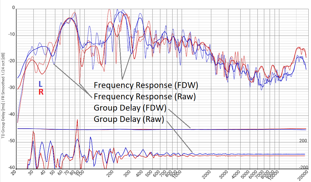
The “Group Delay (FDW)” curve shows the same measurement data on the same scale, but with frequency-dependent windowing FDW (see later). The value range of perhaps 20 ms is just about recognizable but certainly much more meaningful.
For further investigation, I (as the author of the app and documentation) played bursts in the 80 Hz range and compared the oscillograms with those of the microphone signals. Because some singularities in waves are related to nonlinearities, I looked at the actual physical microphone signal instead of a calculated convolution of these bursts with the impulse response.
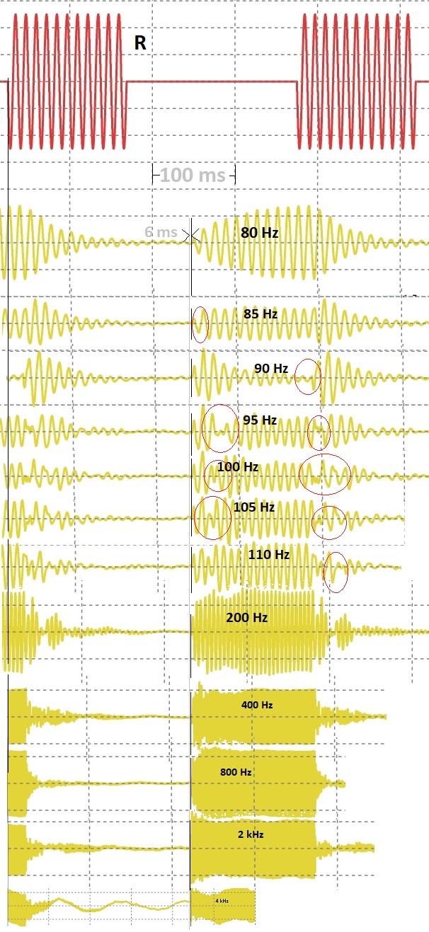
Bursts, played back and recorded with Hifi apps Car Audio Setup. Red: Played burst (only shown for 80 Hz). Yellow: Microphone signals of all frequencies. The beginnings were always aligned at the same distance from the respective signals played back (hence the jumps in the grid) and marked with a thin black line. The vertical gray line 6 ms in ahead is for orientation only.
It is immediately apparent that the beginnings of the bursts shift by a few ms at most; shifts on the order of the unwindowed GD are, as expected, inconceivable. However, the origin of this effect can still be seen: the phase jumps at the points circled in red. It stands to reason that, as with the excess phase (see above), the cause can be found in the additive interaction of the transfer functions of the room. However, the total phase is calculated according to the phase of all signal components of the respective frequency arriving (at some point). The GD is in turn calculated from the change in this total phase per frequency change. Accordingly, a significant jump appears in the result. Technically speaking, the frequency of the envelope is so close to the carrier frequency that the "transportation time" of the wave packet is no longer described (see later).
For the sense of hearing, however, this effect plays a completely different role than the first arrival time of the first direct sound (thin black lines): The latter is crucial for time-based localization of the sound source. And we are probably the descendants of those who mastered the transit time-based localization of a roaring tiger, regardless of any reflections and phase shifts. This can and should be taken into account in the calculation by looking only at the first wave trains of the measurement (if not the black line, then at least). This, in turn, is the main idea behind FDW.
However, it is also clear that the measurement result without FDW is not worthless. The peak indicates a clear acoustic peculiarity, albeit possibly due to enriching indirect sound. You could now play sounds at this frequency, walk around the room, and check whether this peculiarity was previously perceived as disturbing and, if necessary, improve the situation. A quantitatively meaningful result can only be obtained after FDW. This is also used as the basis for digital room correction (DRC). The prevailing opinion [Barnett 2017] is that DRC must be based on measurements with FDW. For simple adjustment tasks such as the delay of a subwoofer, however, the smoothed version without FDW is perfectly adequate.
Details and possible points of criticism
Criticism: The evaluation was carried out graphically using the measured oscillograms, and the start times were drawn subjectively at the first visible oscillation.
In the calculation below, for example, the GD is not this beginning, but the point of the half rise.
My answer: This may be common in signal theory, but it does not take into account the logarithmic perception of the sense of hearing and the importance of the first direct sound. The thesis
"perception begins as soon as you see something on the oscillogram" is certainly not perfect, but it is closer to reality.
In addition, the values would practically only change significantly up to the 85 Hz measurement, and almost not at all at the neighboring points up to 110 Hz.
Criticism: The measurement should be replaced by the mathematically correct variant "Convolution of the impulse response with the bursts".
My answer:
I have done this and there are no visible differences. The calculation of the somewhat strange-looking 90 Hz oscillogram compared to the measurement above:
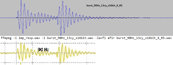
The effects therefore also occur in linear, time-invariant systems and the cause is not to be found in non-linearities.
Even more measuring points would not provide any new insights. Basically, two points would be enough to show the discrepancy in the values.
Criticism: The bursts are not windowed, so the measurement is correspondingly inaccurate.
My answer: Certainly much more accurate than the 500 ms found. The room and loudspeaker provide a certain windowing anyway and the wave trains with the frequencies to be examined are clearly visible in the oscillograms,
The influence of the harmonics of the circumscribing rectangle can therefore not be too strong.
Detail: FDW settings for the relevant frequency range: 34-59 Hz: 132 ms Window width (je 25 ms rise / fall), 59-103 Hz: 96 ms (21 ms), 103-179 Hz: 72 ms (18 ms), i.e. at the lower limit of what is usual (very short windows).
Question: What accuracy can be expected from a GD measurement?
My answer: With reasonably selected FDW parameters, hopefully in the range of the perception threshold of the sense of hearing, but not much better.
Basically, you would have to look at the oscillograms of different frequencies individually (automatically?) and compare them with your knowledge of psychoacoustics.
If you calculate a DRC from the measured phase, you should simply carry out various evaluations and look for the best result using a listening test.
Size of Time Windows for Digital Room Correction
Digital room correction (DRC) generated with hi-fi apps is discussed in detail elsewhere. Unlike a classic equalizer, it not only allows you to influence the frequency response, but also to specifically control the temporal behavior of individual frequency ranges. However, the aspect of which frequency ranges should be “observed for how long” for correction is so closely related to GD that it will be discussed here.
The following explains which parts of the time domain should be corrected and which should not, and how to deal with the inevitable gray area between the two. As discussed above, uncritical, complete correction of all timing errors would result in a system that sounds worse than uncorrected. The appropriate length of an FIR DRC filter scales primarily with the wavelength of the respective frequency to be corrected and the resolution to be achieved at that frequency. A FIR of 200 ms is short for 50 Hz, but extremely long for 2 kHz. The technically important total length of the filter depends on the lowest frequency. Narrowband corrections force long time windows, so it is highly questionable whether, for example, the approximately 5 Hz wide peak at 80 Hz should be corrected in the measurement.
Correcting irregularities such as the areas circled in red in the measurement would certainly be wrong. They are caused by random overlaps of several reflections at the exact location of the measuring microphone. Even minimal changes in position—significantly smaller than the distance between the ears—lead to significantly altered measurement values, although the perceived sound image remains largely stable overall. A correction function based on this would most likely degrade the signal at the slightly shifted listening position.
On the other hand, it would not be effective to keep the length of the FIR correction so short that only the position-independent part is addressed: Sound travels approximately one meter in 3 ms. In a listening room with a 3 m difference in distance between direct sound and sound reflected from the wall, this would correspond to approximately 9 ms in geometric acoustics. In other words, 9 ms after the start of the sound event, the reflected sound also reaches the ear. At frequencies around 100 Hz, this is less than the period duration, so measurements (and corrections based on them) in this range are subject to error. On the one hand, they contain the desired position-independent effects (transient processes, time errors, reflections in the speaker cabinet), and on the other hand, they contain the aforementioned reflections, which our sense of hearing copes with better without treatment. However, these effects cannot be distinguished in a measurement with an omnidirectional microphone. In a perfect world, the side walls, ceiling, etc. would be removed for the duration of the measurement. In the real world, reflections should be treated acoustically from the outset, e.g., in such a way that [EBU 3276] is fulfilled.
However, experience shows that DRC still works at 20 Hz = 1/50 ms. At 20 Hz, the wavelength is 17 m, so the chaotic pattern of interference at 100 Hz is not to be expected here. Instead, a much slower time response is to be expected, i.e., compromises must be made when correcting the GD in order to minimize side effects (preringing). In other words, a large measurement window is required for this frequency range, but the DRC should focus more on the frequency response and less on the GD. An intuitive picture of such differences, together with a frequency-dependent sound field measurement, is helpful when experimenting with different windowing.
There is a proposal to equalize only the speakers. Older speakers that are fundamentally good but still have little phase equalization could benefit from this. Free-field measurements (in the garden) could form the basis for this. However, this does not take into account any asymmetries in the room, which will ultimately probably lead to a poorer stereo image.
How long should the correction be for a specific frequency range? For live events, the answer is simple: you have to work with 1024, maximum 4096 taps (at 48 kHz) to keep the delay below 100 ms. DRCs of this length are therefore also useful. However, a concert hall also has other room modes. For home playback, the delay is irrelevant, and a longer DRC results in better frequency sharpness (see table below). This, in turn, is a prerequisite for capturing the various frequency components of a loudspeaker's direct sound with sufficient precision for correction. And their temporal coordination is, in turn, a prerequisite for good sound definition: The nerves in the cochlea fire extremely quickly to encode sounds. The outer hair cells move up to 20,000 times per second (=1/50 µs). Perception times for temporal accuracy can actually be well below the values given above, e.g., at 35 µs when several sounds are played together in a kind of chord—see, for example, the introduction to [Møller 2007] for an overview. However, the results of scientific studies cannot be applied 1:1 to the requirements of DRC: They refer to specific signals, often noise or bursts, not music, and were often measured using headphone experiments. Ultimately, it is sufficient to know that the desired correction should be as accurate as possible. The answer to the question at the beginning is therefore “as long as possible for the respective frequency due to reflections in order to capture the phase response of the first direct sound as accurately as possible.” The result can sometimes be zero, for example, if the distribution of reflections is very unfavorable.
In addition to reasonable upper limits, there are also absolute lower limits. If these limits are not met, a DRC is not bad, but pointless: It is not possible to determine the period duration of a flashing light from a video that only contains one turn-on process. Similarly, it is not possible to deduce all the frequency components of a longer period from a small piece of a sound wave. At least one complete period is required, in practice more likely two, or five in the case of a settling subwoofer, and sometimes ten to study the behavior at a specific frequency for a reliable measurement of the entire spectrum. However, as the image with the recorded bursts (above) shows, there should not be too many periods due to the aforementioned reflections. Ultimately, only position-independent effects (settling processes, time errors, reflections in the speaker enclosure) should be corrected at the beginning of a sound event, but this correction should be as accurate as possible. Together, this results in the following rules (not laws of nature)
- To put it plainly: if +3dB is measured at listening position one and -5dB at listening position two, either the measurement window is too large or the listening room is not sufficiently insulated. In any case, DRC based on this data is pointless.
- More generally: The time window for correction should be determined based on how position-dependent the amplitude and phase are in its frequency band: At the latest when the differences between the listening positions fall within the correction range, the window is too large.
- If the damping is very poor, the maximum window size for some frequencies may also be zero.
- FDW should be viewed as “position-constancy-dependent windowing.” Position constancy is the decisive value, which in turn depends on the frequency.
- Corrections in the bass range (below 200 Hz) require FIR lengths of over 100 ms, and the benefit is highly dependent on position.
- The sample configurations in [DRC Sbragion] specify 250 ms (“minimal”), 500 ms (“normal”) or 544 ms (“strong”) for the minimum phase portion of the correction at 20 Hz, and 1/1000 of that at 20 kHz (i.e., 1000 times the value). However, the values in between do not necessarily have to be geometric (20 Hz 250 ms; 200 Hz 25 ms ...). This allows you to use the intuitive image of the wave field in the respective listening room described above to make the correction in the middle range shorter or longer as desired. For the remaining excess phase, the values for 20 Hz are 10.4, 21.3, and 22.7 ms.
- Some “single-button systems” that can be operated without prior knowledge limit the correction to 200–300 Hz for robustness reasons.
- For corrections in the fundamental frequency range of 200–800 Hz, FIR lengths in the range of a few milliseconds are useful.
- For corrections in the range above 800 Hz, very short FIRs are sufficient; phase correction is usually uncritical.
- Narrowband resonances should be treated better by room design and, if that is not possible, by amplitude.
- A practical rule for FDW is “five to twenty wavelengths.”
Lower Limit of Time Windows for Digital Room Correction
One value for the smallest possible time window is the period duration $1/f$; shorter corrections are physically meaningless. The formulas for estimating the GD provide another criterion for the minimum lengths of filters: The basic idea is that the filters are identical to the transfer function, only with swapped zeros and poles. This allows the quality factor, phase, and GD to be calculated based on the specified frequency and the desired bandwidth. The model system is the IIR (Infinite Impulse Response) of a second-order all-pass filter, and the transfer function is set as a quotient. FIR filters must be designed significantly longer, perhaps 5 to 10 times longer, to achieve comparable results. Without this heuristic factor, the following values are obtained for $\tau_{gr, ap 2}(\omega_0)$ and $\tau_{gr, ap 2}(\omega \rightarrow 0)$:
| $f_0$ [Hz] (1/f [ms], # Sam 48k) | 20 (50, 24k) | 50 (20, 9600) | 100 (10, 4800) | 200 (5, 2400) | 500 (2, 960) | 1k (1, 480) | 2k (0.5, 240) |
| Q=0.67 (N=1 Oct) | |||||||
| Q=1 (N=1.39 Oct) | |||||||
| Q=2 (N=0.71 Oct) | |||||||
| Q=3 (N=0.48 Oct) | |||||||
| Q=5 (N=0.36 Oct) | 79.58 ... 159.15 | 31.83 ... 63.66 | 15.92 ... 31.83 | 7.96 ... 15.92 | 3.18 ... 6.37 | 1.59 ... 3.18 | 0.80 ... 1.59 |
| Q=7 (N=0.36 Oct) | 111.41 ... 222.82 | 44.56 ... 89.13 | 22.28 ... 44.56 | 11.14 ... 22.28 | 4.46 ... 8.91 | 2.23 ... 4.46 | 1.11 ... 2.23 |
| Q=10 (N=0.144 Oct) | 159.15 ... 318.31 | 63.66 ... 127.32 | 31.83 ... 63.66 | 15.92 ... 31.83 | 6.37 ... 12.73 | 3.18 ... 6.37 | 1.59 ... 3.18 |
| Q=15 (N=0.096 Oct) | 238.73 ... 477.46 | 95.49 ... 190.99 | 47.75 ... 95.49 | 23.87 ... 47.75 | 9.55 ... 19.10 | 4.77 ... 9.55 | 2.39 ... 4.77 |
| Q=20 (N=0.072 Oct) | 318.31 ... 636.62 | 127.32 ... 254.65 | 63.66 ... 127.32 | 31.83 ... 63.66 | 12.73 ... 25.46 | 6.37 ... 12.73 | 3.18 ... 6.37 |
The first line specifies various frequencies, $1/f$ in ms is the corresponding period duration, shorter corrections are physically meaningless and are crossed out in the following lines. “# Sam 48k” is the corresponding number of samples at a sampling frequency of 48 kHz. The bandwidth as frequency difference $BW=f_0/Q$ results from the width of the peak in the frequency response at half power, i.e., -3 dB or $1/\sqrt{2}\simeq 70\%$ of the amplitude. The bandwidth in octaves is calculated from $N=\ln(f_2/f_1)/\ln(2)$, where $f_2$ and $f_1$ are the upper and lower cut-off frequencies of the band read at -3 dB. The conversion to quality is performed using the formula $Q=\sqrt{N}/(2^{N}-1)$ [sengpielaudio].
So, for example, to correct the resonance at 80 Hz with a bandwidth of approx. 5 Hz examined in the measurement above, one could use $N=\ln(82.5/77.5)/\ln(2)\simeq0.1$, i.e. Q=15. According to the next-to-last line, the value for the GD is between 95.49 and 190.99 ms, which is slightly lower than the values of the unwindowed GD in the plot, but within the expected range. A shorter filter length would be physically meaningless, and there is also the "significant" factor of 5..10. It would therefore be necessary to check whether the measurement results at this window length behave at least similarly at all listening positions, so that a correction moves all of them in the desired direction. This is probably not the case. In practice, smaller values between 5 and 20 wavelengths are often chosen, i.e., 62.5 to 250 ms for this frequency. For these reasons, sharp room resonances of the type shown are rarely treated with phase corrections.
In loudspeaker construction, quality factors $Q_{ts}$ in the range of 0.3 to 0.5 are used—perhaps 0.6 for closed systems. The values of the required correction durations are therefore in the range of the crossed-out first row of the table, meaning they should have at least a few period durations of the respective frequencies.
For Technicians
By Fourier transforming the transfer function of a linear time-invariant system, a time shift (delay) $\tau_{d}$ becomes a frequency-proportional phase shift: $\mathscr{F}\{ F(\omega)\} = f(t) \Rightarrow \mathscr{F}\{\exp(i \omega \tau_{d}) F(\omega)\} =f(t-\tau_{d})$ where $\omega$ is the angular frequency and $t$ is the time. In other words, in this simple case the transfer function can be taken as $H(\omega)=k\exp(-i \omega \tau_{d}) $ i.e. $$ \begin{align} |H( \omega)| &= k \\ \angle H( \omega) &: = \varphi(\omega) = -\omega \; \tau_{d}\\ \end{align} $$ Due to the linear relationship between $\omega$ and $\angle H(\omega)$, the delay can therefore be written as both a fraction and a differential quotient: $$ \tau_{d} = - \frac{ \varphi( \omega)}{\omega} = - \frac{ \mathrm{d}\varphi( \omega)}{\mathrm{d}\omega} $$ The delay is not frequency-dependent; there is no such thing as a frequency-dependent delay. The phase increases linearly with time; the filter is linear phase. A delay can only be defined for linear phase filters. However, it may still be useful to separate a linear phase component from any filter based on subjective criteria, e.g., to synchronize image and sound as well as possible. $\tau_{d}$ is simply the time it takes for the signal to reach the receiver. In simple terms, the equation states that if a wave train of a certain frequency is required to bridge a certain distance, then two wave trains of double the frequency are required.
In the real world, e.g., a bass reflex channel that oscillates at a certain frequency, this simple relationship is naturally lost. The additional frequency dependence is reflected in a distortion of the wave train. Frequency-dependent propagation times are added to the frequency-independent delay. $|H(\omega)|$ can still be assumed to be constant in the narrow frequency range under consideration.
${ \mathrm{d}\varphi( \omega)}/{\mathrm{d}\omega} $ now depends on the respective frequency $\omega_0$ under consideration. The immediate vicinity of the respective $\omega_0$ or the first term of the Taylor expansion around $\omega_0$ is relevant for the GD. A narrow frequency band is always considered; a single frequency has no time behavior. As mentioned at the very beginning, the common and certainly useful formulation of the propagation velocity of "a specific frequency" is technically meaningless. $$ \begin{align} \angle H( \omega) &= \exp\Big(i \varphi(\omega_0) + i (\omega-\omega_0) \varphi'(\omega_0) \Big) \\ &= \exp\Big(i \omega_0 \underbrace{\varphi(\omega_0)/\omega_0}_{-\tau_{ph}} \Big) \exp\Big(i \underbrace{(\omega - \omega_0)}_{\Delta \omega} \underbrace{\varphi'(\omega_0)}_{\to - \tau_{gr}} \Big) \end{align} $$ The constant term of the development, or the first $\exp(\cdot)$ multiplier in the second line, also loses its meaning as a pure delay, since the new generalization now allows the delay time to be frequency-dependent. This is why we now refer to a phase delay. $$ \tau_{pd}(\omega) = -\frac{ \varphi(\omega)}{ \omega} \\ $$ The second factor can be clearly seen as the propagation of a beat, which is much slower than $\omega_0$ due to the small $\Delta\omega$. In a frequency-modulated radio station, $\omega_0$ would be the carrier frequency, e.g., 100 MHz, and $\Delta\omega$ would be characterized by the transmitted music, e.g., a maximum of 15 kHz. $\tau_{gr}$ describes the time required by the envelope of a signal with a narrow frequency range around $\omega_0$, which is not the time required by the signal itself. Since most of the energy is in this range, the potentially misleading term (see above) "energy delay" is used in addition to "envelope delay". $$ \tau_{gr}(\omega) = -\frac{\mathrm{d} \varphi(\omega)}{\mathrm{d}\omega} \\ $$ However, it still makes sense to split $\tau_{pd}$ into a trivial component describing the time shift and the (usually decisive) component that determines the frequency dependence of the system through resonances, filter effects, etc. Software for displaying GD therefore offers an "unroll function" that allows automatic or manual deduction of a linear phase component. This gives the user the ability to view the system behavior determined by resonances, filter effects, etc. without disruptive phase shifts.
As shown above, the slow progression of the envelope must be ensured by appropriate windowing when measuring room acoustics. Otherwise, $\tau_{gr}$ does not reflect the common definition "...how long it takes for a certain frequency to be reproduced..." If a signal with a carrier frequency $\omega$ is applied, which is modulated by a sufficiently slow envelope, then $\tau_{gr}$ and $\tau_{pd}$ are divided accordingly during transmission: $$ x(t) = \underbrace{ m(t)}_{\text{ Enveloping curve }} \underbrace{ \cos(\omega t)}_{\text{ Carrier freq }} \longrightarrow \underbrace{ m(t-\tau_{gr} )}_{\text{ Enveloping curve }} \; \underbrace{ \cos(\omega (t- \tau_{pd} ))}_{\text{ Carrier freq }} $$ A pure phase delay $\tau_{pd}$ can be accommodated in the cos term as described above, the crucial remainder shifts the envelope depending on which frequency it envelopes. The frequency-dependent change in amplitude was omitted for simplicity.
Rule of Thumb for Estimating the GD
Im APPENDIX 1 of [Møller 2007], the phase behavior and group delay of first- and second-order all-pass filters are explicitly calculated. For the first order, the authors start with $$ H_{ap 1}(\omega) = \frac{\omega_0-i \omega}{\omega_0+i \omega} $$ where $H$ is the transfer function and the frequency $\omega_0$ is given by its pole and zero. Both the numerator and the denominator can be viewed like a phase diagram; both have the same phase angle $\tan^{-1}(\omega/\omega_0)$. The phase angle of the entire system $\varphi(\omega)$ therefore has twice the value. This means that $$ \tau_{ph, ap 1}(\omega) = \frac{2 \tan^{-1}(\omega/\omega_0)}{\omega}; \;\; \tau_{gr, ap 1}(\omega) = -\frac{2 / \omega_0}{1+(\omega/\omega_0)^2} \\ \\ $$ With an analogous calculation for a second-order allpass filter, a relationship between quality and GD can be established. It is $$ H_{ap 2}(\omega) = \frac{(i \omega)^2-i \omega (\omega_0/Q) + \omega_0^2 }{(i \omega)^2+i \omega (\omega_0/Q) + \omega_0^2 }, $$ where $Q$ is the quality factor. Phase and GD are calculated analogously to the first-order allpass filter. For the section Size of Time Windows for Digital Room Correction, the peak of the GD at $\omega_0$, its relationship to the bandwidth of resonances, and the limit value at low frequencies are decisive. For modes with high quality factor $Q>0.5$, $$ \tau_{gr, ap 2}(\omega_0) = \frac{4Q}{ \omega_0}; \;\; \tau_{gr, ap 2}(\omega \rightarrow 0) = \frac{2Q}{ \omega_0} $$ where the first equation represents the peak of the GD.
Numerical Calculation
In discrete-time transmission systems, as represented by digital signal processing, the discrete GD is related to the sampling interval $T$: $$ \frac{\tau_d(\Omega)}{T} = - \frac{\mathrm{d}\,\operatorname{arg}\{H(e^{i\Omega})\} }{\mathrm{d}\Omega} $$ with the angular frequency $\Omega$ normalized to the sampling frequency $f_s$: $$ \Omega = \frac{\omega}{f_\mathrm{s}} = \omega \cdot T $$ The advantage of the normalized form in discrete-time systems is the independence from concrete sampling frequencies.
Example
Let the transfer function of a discrete system be an averaging over the first 5 indices, i.e. $$ \begin{align} h[n] &= \frac{1}{5} (\delta(n) + \delta(n-1) + \delta(n-2) + \delta(n-3) + \delta(n-4)) \\ H(\Omega) &= \frac{1}{5} (e^{-i0} + e^{-i\Omega} + e^{-i2\Omega} + e^{-i3\Omega} + e^{-i4\Omega} ) \\ &= \frac{1}{5} ( e^{i2\Omega} + e^{i\Omega} + e^{0} + e^{-i\Omega} + e^{-i2\Omega} ) e^{-i2\Omega} \\ &= \frac{1}{5} ( 2 \cos(2 \Omega) + 2 \cos( \Omega) +1) e^{-i2\Omega} \\ \end{align} $$ The cos terms in the brackets (the amplitude response) are real, only the last multiplicand has influence on the phase. Consequently the group delay becomes $$ \tau_{\rm gr}(\Omega) = - \frac{\mathrm{d}\varphi(\Omega)}{\mathrm{d}\Omega} = - \frac{\mathrm{d} (-2\Omega)}{\mathrm{d}\Omega} = 2. $$ This can be understood if you imagine a step function as a signal, which jumps at $t=t_0=0$ from 0 to 1. When the signal reaches the system, at $t<0$ the output becomes 0, then at $t=0, 1, 2, 3, 4$ to$1/5$, $2/5$, $3/5$, $4/5$, $1$, i.e. after the group delay time the mean of the flank is reached.By the way, the example is a linear phase filter: the phase includes only the $\arg \exp(-i2\Omega)$ term. Roughly speaking, this ultimately comes from the symmetrical structure of the 5 coefficients. While linear-phase filters usually have their maximum in the middle of the impulse response due to this symmetrical structure, the minimum-phase version of the same filter (with the same amplitude response) has the largest coefficients at the beginning of its impulse response. On [falstad.com] different filters can be simulated.
Some measuring devices can calculate (approximate values for) the group delay (directly) from two phase measurements at neighboring frequencies The app "Subwoofer Optimizer" determines the transfer function via logsweep, which is evaluated with Farina's algorithm. The group delay is determined (after smoothing) from the differential quotient of the phase.
References
[Barnett] Mitch Barnett: Accurate Sound Reproduction Using DSP. Independently published (2 April 2017) ISBN-10 : 1520977905 ISBN-13 : 978-1520977904
[Blauert 1978] Blauert, J. and Laws, P: "Group Delay Distortions in Electroacoustical Systems" Journal of the Acoustical Society of America Volume 63, Number 5, pp. 1478-1483 (May 1978)
[Burkowitz, Fuchs 2009] Peter K. Burkowitz, Helmut V. Fuchs "Das vernachlässigte Bass-Fundament" Vereinszeitschrift des Verbands Deutscher Tonmeister 2/2009 p. 35
[EBU 3276] Listening conditions for the assessment of sound programme material: monophonic and two–channel stereophonic. EBU Tech. 3276 – 2nd edition https://tech.ebu.ch/docs/tech/tech3276.pdf May 1998
[Earl Geddes] mehlau.net/audio/multisub_geddes
[Earl Geddes - YouTube] Earl Geddes on Multiple Subwoofers in Small Rooms https://www.youtube.com/watch?v=SCWL-zusyqw
[falstad.com] "...some educational applets I wrote to help visualize various concepts in math, physics, and engineering..."
http://www.falstad.com/mathphysics.html
http://falstad.com/dfilter/
[Goertz 2001] Goertz A, Wolff M (2001) "Neue Methoden zur Anpassung von Studiomonitoren an die Raumakustik mit Hilfe digitaler Filterkonzepte" Teil 1 von 2. Fortschritte der Akustik, DAGA 2002 http://www.ifaa-akustik.de/files/DAGA2002-Teil1.PDF http://www.ifaa-akustik.de/files/DAGA2002-Teil2.PDF
[Goossens] Sebastian Goossens "Wahrnehmbarkeit von Phasenverzerrungen" Institut für Rundfunktechnik, München https://forum2.magnetofon.de/bildupload/goosphase.pdf
[Grätz 1928] L. Grätz "Die Elektrizität und ihre Anwendungen" Jengelhorns Nachf. Stuttgart, 1928
[Møller 2007] Møller, Henrik and Minnaar, Pauli and Olesen, Søren and Christensen, Flemming and Plogsties, Jan "On the Audibility of All-Pass Phase in Electroacoustical Transfer Functions" J. Audio Eng. Soc., Vol. 55, No. 3, pp 115-134 (March 2007)
[MSO] Multi Subwoofer Optimizer, Andy C https://www.avsforum.com/threads/optimizing-subwoofers-and-integration-with-mains-multi-sub-optimizer.2103074/
[Münker 2016] Christian Münker: "DSP auf FPGAs: Kap. 5-2 Do-It-Yourself FIR Filterentwurf" https://www.youtube.com/watch?v=y0PNXUI5x1U
[sengpielaudio] "Bandpassfilter (BPF) und EQ-Filter - Beziehung zwischen Q-Faktor und Bandbreite B " https://sengpielaudio.com/Rechner-bandbreite.htm
[Welti Devantier] Todd Welti, Allan Devantier: Low-Frequency Optimization Using Multi Subwoofers. Harman International Industries Inc. Northbridge CA 91329 USA, Manuscript received 2006
[Welti Harman] Subwoofers: Optimum Number and Locationsby Todd Welti Research Acoustician, Harman International Industries, Inc.twelti@harman.com multsubs_0.pdf links folien rechts text Seite 4 "Multiple Subwoofers != Multiple Subwoofer Channels"
Forendiskussion. Aktuell (Okt 2020) 234 Seiten. https://www.diyaudio.com/forums/subwoofers/134568-multiple-subs-geddes-approach-149.html
Eine Art Review mit Raummoden, Welti, Geddes etc. Subwoofer / Low Frequency Optimization By Amir Majidimehr [Note: This article was published in the May/June 2012 issue of Widescreen Review Magazine]